Model Predictive Control
IIA4117,
Fall 2025, University of South-Eastern Norway, Campus
Porsgrunn.
This is an advanced control course that is offered to the
master students at the University of Southeastern Norway. The course is taught
in the fall semester every year. The language used for teaching is English.
This is the official homepage of the course. In this
page, the students can find the videos, lecture notes, exercises, project work
description and other necessary documents and files used in the course.
Important
note: Canvas will be used only for submission of the tasks
(lab journals, reports, source codes etc.) by the students.
Many of the videos are recorded live during the classroom
while the teaching session is going on. The videos are recorded with the hope
that it will provide a basis for the students to watch the whole lectures
(multiple times) outside the teaching hours.
|
Instructor: Roshan Sharma, PhD, Associate Professor email: roshan.sharma@usn.no
, room: B-250b Study point: 5
credits Exam:
Written final exam (60%), project work (40%) |
Information about the
course, exam, project work, learning outcomes, expectations from this course
etc. |
|
|
Download
lecture notes as pdf Download
previous exams-solutions here NEW: Suggested
Solution for 2024 final exam About group project work: Choice 1: (Download
group project description here – Lab Helicopter Unit) Choice 2: (Download
group project description here – Oil well drilling) Note: For the group project work, there are two choices
(two case studies). Each group must select ONLY ONE between these two
choices, and work with the group project work. Deadline for the submission of
the report for the project work is 20 November,
kl. 23:59. Please submit your group
project report in Canvas. One report per group. |
The following table lists the course syllabus and all the
links to videos and other documents
|
Dates |
Description |
Links
to videos |
|
|
Preliminary requirements |
Install
Simulink/MATLAB in your computers/laptops at home before coming to the first
lecture. The installation
key for MATLAB/Simulink will be sent to your USN student email address. |
||
|
Lecture 1: Week 33 Aug. 14 (Room A289) Time:
09:15 – 12:00 |
|||
|
Brief Introduction |
|||
|
Revision on dynamic
models: Different types of dynamic models suitable for optimal control. |
|||
|
Linearization of
nonlinear models |
|||
|
Example of dynamic
model + linearization + discretization: ·
Inverted pendulum model, process description ·
Linearization of pendulum model ·
Integration/Discretization |
|
||
|
Simulation of
dynamic models in Simulink: ·
Openloop simulation of nonlinear model of Inverted Pendulum using Simulink, download simulator
here ·
Real-time simulation of nonlinear model of
Inverted Pendulum using Simulink, download simulator
here (run the file IVP_real_time.slx) ·
Openloop simulation of linear model of Inverted Pendulum
using Simulink, Download real-time pacer files here |
|
||
|
LabWork 1: Week 34 Aug. 21 (Room A289) Time:
08:30 – 12:00 |
From this year there will be two case studies for group
project and hence two case studies also for labwork
1. Please choose ONE of them (no need to do both of them for
labwork 1). (ii) If you will choose “oil well drilling” as group
project work later on, then choose case study 2 for labwork
1 now. Case study 1: Simulation of
dynamic model of two degrees of freedom (2DOF) helicopter model in Simulink (Doing this labwork 1 will help you in your project work.) |
|
|
|
Description of the
helicopter unit + mathematical model of 2DOF helicopter |
|||
|
Explanation of the real unit
by the teacher in the classroom |
|
||
|
Labwork
tasks, download it
here for case study 1 |
|
||
|
Case Study 2: Simulation of Oil well drilling Download the labwork description here for case study 2 |
|
||
|
Description of
the oil well drilling process Inspiration 1: Here is a video of a simulator for performing openloop simulations for the oil well drilling process
for pipe connection procedure. |
Openloop-simulation-demo-Drilling |
||
|
Some useful videos you can see
before starting labwork tasks |
|||
|
Info: Submit a lab journal with your
implementation in canvas
(screen shots of your implementation + little description of your results) Deadline: Sep 4, 2025 (kl. 23:59)
for campus students,
Sep. 11, 2025 (kl. 23:59) for online students |
|
||
|
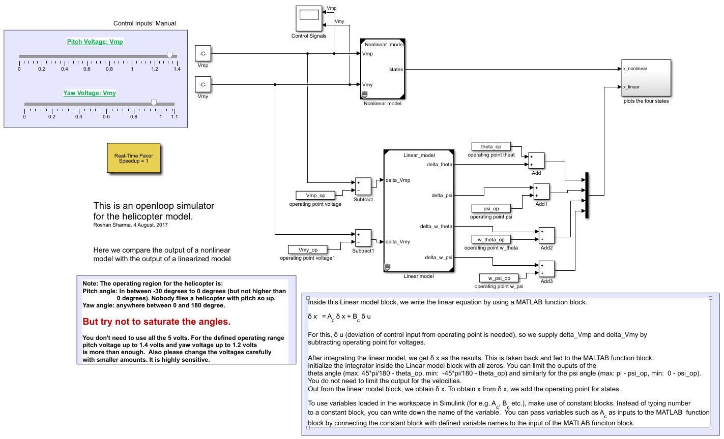
Inspiration 2: This is how
the helicopter case study implementation looks like. See
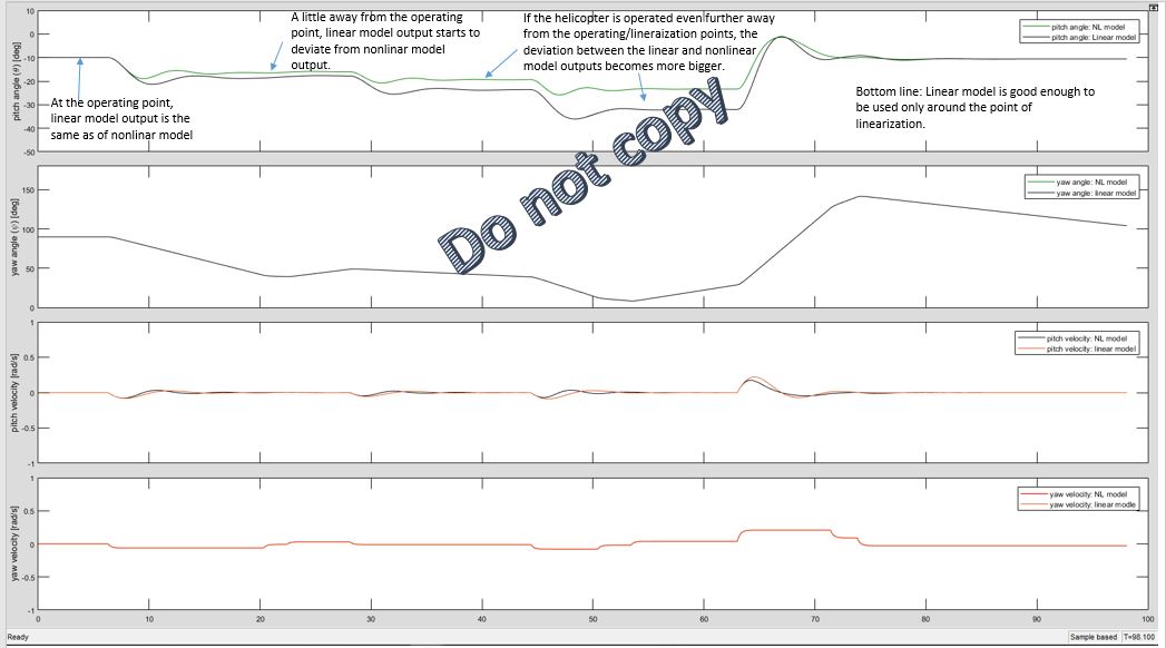
here. Inspiration 3: This is how the comparison of
the linear vs nonlinear model of lab helicopter looks like. See
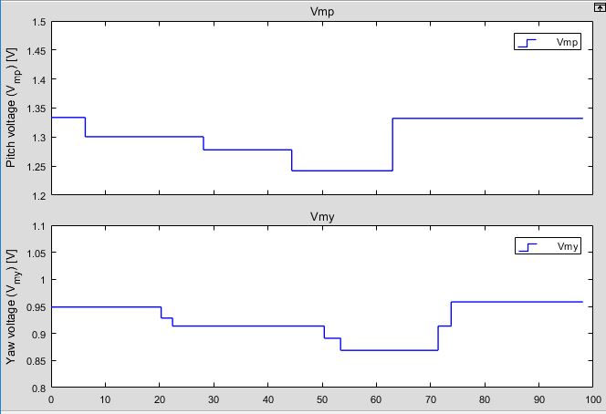
here. Inspiration 4: This is the control signals plots for lab
helicopter unit. See
here. From the picture you can see that you don’t need to use too high
voltage values. |
ß Please look at these links to see
how the implementation should look like together with expected results. |
||
|
Lecture 2: Week 35 Aug. 28 (Room A289) Time:
08:30 – 12:00 |
Introduction: the
connection |
||
|
Introduction to
mathematical optimization, different types and their general formulation
(objective functions, constraints and bounds). |
|||
|
Let’s first look
into static optimization to get us started. Example: Optimal
operation of oil refinery. ·
Oil refinery, process description ·
QP problem formulation ·
Converting to standard QP form/structure |
|
||
|
Solving oil
refinery QP problem using qpOASES: a) Pre-requirements: ·
Installation of solver qpOASES, download qpOASES here
· From 2017b and newer version of MATLAB,
please download
this compiler here (Right click on the download
link and choose ‘save link as’. Save it to a desired location in your PC.
Just double click it after downloading and follow the instructions on the
screen) ·
Testing/Compilation of qpOASES b) Solving refinery
problem in Simulink |
|
||
|
Dynamic optimal
control and performance index, concept of prediction horizon, Linear
Quadratic (LQ) optimal control |
|||
|
Exercise 1: static optimization (to help you learn how to use qpOASES in Simulink) |
|
||
|
Info: Submit a lab journal with your
implementation in canvas
(screen shots of your implementation + little description of your results) Deadline: Sep. 11, 2025 (kl. 23:59)
for campus students,
Sep. 18, 2025 (kl. 23:59) for online students |
|
||
|
Lecture 3: Week 36 Sep. 4 (Room A289) Time:
08:30 – 12:00 |
Useful matrices and
their structure, kronecker product |
||
|
Efficient
formulation of LQ optimal control problem: using Kronecker
product formulation. Handling bounds and
inequality constraints |
Classroom videos |
Videos with software Handling
bounds and inequality constraints |
|
|
Example: LQ optimal
control of inverted pendulum Problem formulation with
linear pendulum model Efficient transformation
into standard QP problem Solution using qpOASES in Simulink Download the simulator
here (After downloading
and extracting: Run the file “LQ_IVP_simulink.slx”).
Point MATLAB to the extracted folder path. |
Please see lecture notes Chapter 3.5.
It also contains codes. Don’t forget to read the comments in between the
codes for more clarification. (Play around with simulator) |
||
|
Exercise 2: Implement your own LQ optimal controller for the linear inverted
pendulum model in Simulink Info: Submit a lab journal with your
implementation in canvas
(screen shots of your implementation + little description of your results) Deadline: Sep. 18, 2025 (kl. 23:59)
for campus students,
Sept. 25, 2025 (kl. 23:59) for online students |
|
||
|
Lecture 4: Week 37 Sep. 11 (Room A289) Time:
08:30 – 12:00 |
The connection |
||
|
Predictive control: ·
Introduction (optimal control
problem vs. predictive control, the difference) ·
The sliding horizon strategy
(introduce the feedback property) (sliding horizon + optimal control problem = model predictive control) |
|
||
|
Example of a racing
car. |
|||
|
Concept about: Warm
Start, Parallel-pool, shrinking horizon strategy |
|||
|
State feedback MPC
and its algorithm. |
|||
|
|
|
||
|
Example of linear
MPC in Simulink: Apply sliding horizon
strategy to LQ optimal control of inverted pendulum to make linear MPC Download the simulink simulator
here (Extract the zip file
to a desired location. Point MATLAB to the extracted folder path. First run
the file “initialization_script.m”. This loads all
the needed parameters and matrices into the MATLAB workspace. Then open the
file “linear_MPC_IVP.slx”.
Play
around by changing the setpoint for x2 (the cart
position). Please also read the comments written in the main simulink file. |
|||
|
Linear MPC in scripting language (e.g. in MATLAB, but same idea also
applies for Python or Julia): Linear MPC in MATLAB + Execution time needed to run linear MPC for
inverted pendulum in MATLAB (for comparison later on in lecture 5) |
|||
|
Exercise 3: (no submission required): By modifying your implementation from
exercise 2 (LQ optimal control), make a linear MPC for controlling the
inverted pendulum? (to
help you learn how to implement sliding horizon strategy). |
|
||
|
Lecture 5: Week 38 Sep. 18 (Room A289) Time:
08:30 – 12:00 |
Reduction of the
size of the LQ optimal control problem |
||
|
a) Lagrangian method |
|
||
|
a) QR factorization |
|||
|
b) Elimination of
unknowns by grouping of control inputs. |
|||
|
MPC with reduced size of the optimal control problem: Example: Linear MPC with reduced size of optimal control for inverted pendulum (comparison of the
execution time needed to run the MPC) |
|
||
|
Feasibility, hard constraints
vs. soft constraints Constraint
relaxation for ensuring feasibility: Slack variables and modified LQ optimal
control problem |
|||
|
Exercise: Continue working with exercise 3 |
|
||
|
Lecture 6: Week 39 Sep. 25 (Room A289) Time:
08:30 – 12:00 |
Formation of
student groups |
|
|
|
The connection: Why
should we estimate the states? |
|||
|
Output feedback
MPC, block diagram , algorithm for output feedback MPC |
|||
|
State Estimation:
Introduction, example |
|||
|
Apriori/ Aposteriori estimates |
|||
|
Kalman Filter Algorithm |
|||
|
Combined State and
disturbance estimation (by augmentation) |
|||
|
Examples and
demonstration: Estimation of states of the helicopter process (simulator)
Estimation of states of the helicopter process (real unit) Download
linear Kalman filter simulator for helicopter
(unzip and open the file linear_Kalman_heli.slx
, run
this file) Download
Unscented Kalman filter simulator for
helicopter just so that you can play around (unzip and open the file UKF_heli.slx , run this file). For your project work, you can design a
linear Kalman filter yourself. Do you see the
difference between the behaviors of these two filters/estimators? Remember: In this
course, we do not learn the theories about Kalman
filters in detail. It is assumed that you know at least about the linear Kalman filter from previous courses. |
|||
|
Exercise (no submission required): Connecting the
real helicopter units to laptops using Simulink. Download the
NI-DAQ-mx and install it on your laptops. If you already have NI-DAQ-mx
installed on your laptops (say for example with LabVIEW), then you don’t need
to install it again. (optional
for year 2025) |
|
||
|
Lecture 7: Week 40 Oct. 2 (Room A289) Time:
08:30 – 12:00 |
Steady state offset, model mismatch, uncertainties, unaccounted disturbances (Lets apply a
linear MPC to the nonlinear model of the plant and see what happens) |
Offset-model-mismatch-uncertainty |
|
|
Integral action,
Offset free MPC: -
Integral action with disturbance model augmentation -
Delta u formulation for integral action -
MPC + I control, adding output
integrators |
Integral-action-dist-model-aug |
||
|
Features of MPC Feasibility,
Stability, Robustness and Implementation |
|
||
|
Improving
Stability: Infinite horizon optimal control, terminal cost, terminal
constraints. |
|||
|
Handling
computational time delay: - As input-output delay - Sampled-data MPC |
Computational-delay-as-io-delay |
||
|
Control hierarchy
and commercial predictive controllers |
|||
|
Exercise:
Continue working with your group project (Download
group project description here) |
|
||
|
|
Nonlinear MPC (seen as a nonlinear
programming/optimization control problem): Nonlinear
optimization: Introduction, nonlinear objectives and constraints Feasible solution,
feasible region (example to plot feasible region), global/local solutions |
|
|
|
|
Convexity and
conditions for optimality |
||
|
|
Active/Inactive
constraints, KKT conditions |
||
|
Week 41 |
Solvers for
nonlinear optimization: MATLAB optimization toolbox (fmincon
solver), OPTI toolbox (open source) Algorithms for
solving NLPs: Sequential Quadratic Programming (SQP), GRG Source
code for the basic general example of a continuous-circulation dryer.
This code shows the basic use of fmincon solver. Unzip the file to a desired location and
run the file dryer_main.m
file. |
|
|
|
Lecture 8: Oct. 9 (Room A289) Time:
08:30 – 12:00 |
Note: The source code explained in the
videos in this section are little bit difficult to read due to screen
resolution. I suggest that you print out the source code and look at it while
watching the videos for this section. At first: Formulation of
nonlinear optimal control problem Simple Example:
Nonlinear optimal control of the pressure at the bottom of a tank (analogous
to drilling operation) Download the MATLAB
source codes here for nonlinear
optimal control problem (unzip and run the file main_file_tankPressure_NL_control.m) Secondly: Nonlinear Optimal control problem + sliding horizon strategy = Nonlinear MPC Use the sliding/receeding horizon strategy to the nonlinear optimal
control problem to make a nonlinear MPC. Simple Example
continued: Nonlinear Model Predictive control of the pressure at the bottom
of the tank ( i.e. application of sliding horizon strategy for the simple
example above) Download the MATALB
source code here for nonlinear MPC (unzip and run the file main_file_tankPressure_MPC.m) |
NL-optimal-control-formulation NL-optimal-control-example-fmincon-tank-pressure |
|
|
|
Improving speed of
nonlinear MPC by control input grouping Download
the MATALB
source code here for nonlinear MPC with control input grouping (unzip and
run the file main_file_tankPressure_MPC_grouping.m) |
See the lecture notes Section 8.8.2 |
|
|
|
Exercise (no submission required): By modifying the NMPC code for the tank
example, design a nonlinear MPC for disturbance rejection. Change the inflow
in your simulation (i.e. introduce disturbance). Is the controller able to
reject the disturbance? |
|
|
|
Lecture 9: Week 42 Oct. 16 (Room A289) Time:
08:30 – 12:00 |
Introduction to
multi-objective optimization (MOO) problems |
||
|
Common methods used
for solving MOO. ·
Weighted sum method |
|
||
|
·
Epsilon-constraint method |
|||
|
·
Goal attainment method |
|||
|
·
Lexicographic or hierarchical method |
|||
|
·
Introduction to evolutionary algorithms |
|||
|
Application of MOO |
|
||
|
·
Water flooded reservoir planning |
|||
|
·
Olive oil extraction |
|||
|
Basic introduction
to Utopia tracking MPC with application to thin oil-rim reservoir |
|||
|
Exercise:
Continue working with your group project |
|
||
|
Oct. 23 |
Continue working with your
group project Deadline for the submission of report for group
project work is 20 November, 2025, kl. 23:59. Please
submit your group project report in Canvas. One report per group should be
submitted. |
|
|
|
Oct. 30 |
Continue working with your
group project |
|
|
|
Nov. 6 |
Continue working with your
group project |
|
|
|
Nov.
13 |
Continue working with your
group project |
|
|
|
(If any group wants to show
the demonstration of applying linear MPC to real lab helicopter units you the
possibility to do so at the campus before the project deadline. But first let
me know by sending me email so that we can plan day/date/time in advance. |
|
||
|
Nov. 20 |
Deadline for group project work
submission in Canvas room |
|
|